Compression, prediction and artificial intelligence

Compression is one of the most powerful concepts in computing. For the normal computer user, compression is associated with making files smaller, so you can store more of them or send them faster over the Internet, but there is much more to it.

An optimal compressor can (or could, if it existed) be used for prediction of the future of a sequence of events (weather, sports, stocks, political events, etc), for example by trying all possible continuations and examine how well it compresses given the history. Conversely, an optimal predictor that gives the correct probability of each possible next symbol can be used for optimal compression by using arithmetic coding.


Compression and prediction

This section on background theory contains possibly scary math and dense prose, but should be understandable for most programmers. Maybe re-read the sentences a couple of times.

Ray Solomonoff has shown [PDF]  that if we let Sk be the infinite set of all programs for a machine M, such that M(Sk) gives an output with X as prefix (i.e the first bits of the output is X), then the probability of X becomes the sum of the probabilities of all of its programs, where the probability of a program is 2 ** (-|Sk|) if |Sk| is the length of the program in bits and "**" means "to the power of". As X gets longer, the error of the predictions approach zero, if the error is calculated as the total squared probability difference.

A technicality is that only those programs count, that does not still produce X, when the last bit of the program is removed.

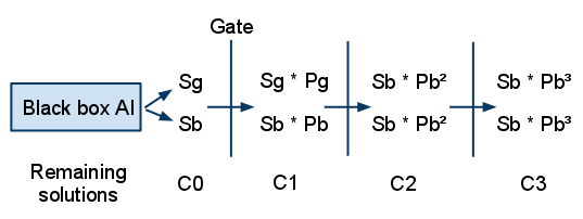
To give a slightly more concrete example, say that you have a sequence of events - a history - and encode those as a sequence of symbols, X. Let us further say that you have a machine, M, that can read a program S and output a sequence of symbols. If you have no further information on your sequence of events, then the best estimate for the probability of a symbol Z to occur next (i.e the best prediction) is given by the set of all programs that output your history X followed by Z. Programs which output X+Z and are short are weighted higher (the 2 ** (-|Sk|) part).

Even more concretely, given the binary sequence 101010101, you wonder what the probability is that the next bit will be 0 given that you know nothing else of this sequence. Sum 2 ** (-program length) for all programs that output 1010101010 vs those that output 1010101011 as their first bits (they are allowed to continue outputting stuff). If we call these sums sum0 and sum1 respectively, then the probability of 0 coming next is sum0 / (sum0 + sum1) and the probability of 1 coming next is sum1 / (sum0 + sum1).

Obviously you cannot find all these programs by just trying every possible program, because 1) they are infinitely many and 2) given the halting problem you cannot in general know if a running program is in an infinite loop or if it will eventually output X.

There is an area of probability theory called Minimum description length, where the language is chosen to be so simple (not Turing complete) so that you can actually find the shortest program or "description". Calculating probabilities this way is very similar to Bayesian probability, but more general.

Solomonoff in (almost) practice

Although the point of the theorem is not to apply it directly in practice, for short sequences X we can actually try. We can avoid problem 1 above, there are infinitely many programs, by generating random programs and see if they produce X. If they do, we count them. This way we can produce an approximation of what the true sum0 and sum1 are. If we set up our random generation such that shorter programs are more likely, then we don't have to bother with the 2 ** (-program length) part and may just have a running count for each sum. If the sequence is too long, this method will be impractical since almost no randomly generated programs will actually output X.

Problem 2 above, when we test programs they may not halt, is harder, but Levin has proposed a way around it. If we in addition to program length use running time (number of instructions executed) as a measure of the probability of our program, we can start by generating all the programs that we intend to test and then run them all in parallel. As our execution moves forward, we will get an increasingly accurate approximation of the true sum0 and sum1, without getting stuck on infinite loops.

If we want to get even more practical, it can be shown that the shortest program that produces X will generally dominate the others and thus it will predict the most likely next symbol. That way you can just search for programs that output X and the currently shortest program will be your best guess. Since we no longer care about the relative probability of the next symbol, but only which is most likely, the search does not have to be random. Thus we can use any method we like for finding a short program. If you search for programs that produce X and find one that almost does, you can construct a "true" solution from that one, by constructing a prefix part that hard codes the places where your original program is wrong. This will produce a longer program, where the length, and thus the "score", is the length of the prefix + the length of your faulty solution. The size of the shortest program that outputs X is called the Kolmogorov complexity of X. The size of the shortest program that outputs X, measured in program size + log(running time), is called the Levin complexity of X.

One way to find these programs is to use genetic programming, just take care that you don't think that you can count the number of programs that produce X and get relative probabilities, because your search will now be skewed towards the solution (and thus its prediction) that you find first.

A small problem is that depending on what machine you choose, i.e which instructions your programs can use and the length of these instructions, you will get different results. The method has a built in bias, since there is no one correct Turing complete language. This difference will however be smaller as X gets longer. One way to understand that is to note that any Turing complete language can emulate any other Turing complete language and that the size of such an emulator is finite. This is called the compiler theorem.

Compression is understanding and the Hutter Prize

When we understand something, we can describe it succinctly. If I have an image of a red perfect circle, the size will be much larger if I describe the individual pixels rather than just say "a red circle of diameter d and thickness t". When I understand what the image is depicting, I can describe it shorter. Sometimes a lossy compression of observed data will actually express the truth better than the exact data. If I take a photo of a red circle, the photo will probably not be perfect, but if I notice what the photo is showing, I can compress it as "a red circle" and some noise which I throw away, and suddenly my lossy compression is a better depiction of the truth.

This equivalence between compression and general intelligence led Marcus Hutter to announce the Hutter Prize, where money is awarded for the best compression of 100 megabyte of English Wikipedia articles. So far the compression algorithms have been impressive (compressing the text to about 15%), but not shown much intelligence or understanding of the articles. When they do start to exhibit some understanding, I think that if they are allowed to compress the data in a slightly lossy way, the first thing that will happen is that some spelling and layout mistakes will be corrected, because these will be surprising to the compressor and thus demand an unusually long representation.

Matt Mahoney has written a good rationale on the Hutter Prize here.

Compression in practice - the juicy stuff

Compression is a powerful tool to measure success and avoid overfitting in a variety of common AI problems. The methods I laid out here are interesting mostly from a theoretical perspective, because of their prohibitively long running times. In my next post, I will expand on my thoughts on how you can use these results to get actual, practical algorithms for common AI problems.

Rescuing a hosed system using only Bash

Prelude
Yesterday I was in a productive mood. "Let's upgrade the ancient Gentoo Linux install on that server that nobody dares to use because the OS is too shoddy", I thought. Since the Gentoo image was from 2005 and never updated, it seemed impossible to upgrade it using normal methods. There were dependencies blocking each other and just an all around awful mess. I downloaded the latest install tarball and decided to just extract it right over the old install. "What is the worst thing that can happen", right?

As it turned out, nothing special happened. It all worked smoothly. Until I ran "emerge" - the package manager for Gentoo. It decided that all those installed packages were quite unnecessary and proceeded to uninstall everything. Everything. Until it could uninstall no more, because it had broken itself.

Challenge
Now I had a system without anything in /bin /sbin /usr/bin, etc. Everything was gone. All that I had left was two remote ssh connections from my desktop which, quite heroically, stayed up despite the best efforts of emerge. I could not open any new connections. The server itself is located on a magical island, far, far away, called Hisingen. I had no intention of making a trip there. Yet.

Ok, what can we do with no binaries?
This is pretty much it:
http://www.gnu.org/software/bash/manual/html_node/Bash-Builtins.html

Notice that such practical commands as "ls", "mv", "ed" and "cp" are not built in. This means that we cannot list or copy files. Or rename them. Or move them. Or edit them. "echo" and "cd" is ok, though. Also we can create new files with echo "blabla" > theFile.

"Bwaha! All I have to do is use tab completion to see what files are in a directory". I chuckled triumphantly to myself, my seductive beard dancing in the wind. Luckily tab completion reported that my /bin/ was full of executables. Unluckily /bin/ was not actually full of executables when I tried to run them. It seems that Bash or Linux or someone had cached the tab completion results.

Since I had the Gentoo tbz-image still in the root directory, all I needed was a way to extract that and I would have all my precious programs back.

Remote file copy

OK.. how do I get bzip2 and tar to the server? Well, using echo "...." > file, it is possible to create new files. But how would you write binary data using echo? It turns out that one can write any byte using \x-hexadecimal escape codes. Unfortunately if you write the zero-byte, \x00, echo terminates. Executables or full of zero-bytes so we need a way to write them too. Well, it turns out that echo can write zero-bytes without terminating using octal escape codes - \0000 will do the trick.

I created a Python program for taking a binary file and convert it to several lines of the type:

> echo -en $'\x6e\\0000\x5f\x69\x6e\x69\x74\\0000\x6c\x69\x62\x63\x2e\x73\x6f\x2e\x36\\0000\x66\x66\x6c\x75\x73\x68\\0000\x73\x74\x72\x63\x70\x79\\0000\x66\x63\x68\x6d\x6f\x64\\0000\x65\x78\x69\x74\\0000\x73\x74\x72\x6e\x63\x6d\x70\\0000\x70\x65\x72\x72\x6f\x72\\0000\x73\x74\x72\x6e\x63\x70\x79\\0000\x73\x69\x67\x6e\x61\x6c\\0000\x5f\x5f\x73\x74\x61\x63\x6b\x5f\x63\x68\x6b\x5f\x66\x61\x69\x6c\\0000\x73\x74\x64\x69\x6e\\0000\x72\x65\x77' > myfile

> echo -en $'\x69\x6e\x64\\0000\x69\x73\x61\x74\x74\x79\\0000\x66\x67\x65\x74\x63\\0000\x73\x74\x72\x6c\x65\x6e\\0000\x75\x6e\x67\x65\x74\x63\\0000\x73\x74\x72\x73\x74\x72\\0000\x5f\x5f\x65\x72\x72\x6e\x6f\x5f\x6c\x6f\x63\x61\x74\x69\x6f\x6e\\0000\x5f\x5f\x66\x70\x72\x69\x6e\x74\x66\x5f\x63\x68\x6b\\0000\x66\x63\x68\x6f\x77\x6e\\0000\x73\x74\x64\x6f\x75\x74\\0000\x66\x63\x6c\x6f\x73\x65\\0000\x6d\x61\x6c\x6c\x6f\x63\\0000\x72\x65\x6d' >> myfile

> echo -en $'\x6f\x76\x65\\0000\x5f\x5f\x6c\x78\x73\x74\x61\x74\x36\x34\\0000\x5f\x5f\x78\x73\x74\x61\x74\x36\x34\\0000\x67\x65\x74\x65\x6e\x76\\0000\x5f\x5f\x63\x74\x79\x70\x65\x5f\x62\x5f\x6c\x6f\x63\\0000\x73\x74\x64\x65\x72\x72\\0000\x66\x69\x6c\x65\x6e\x6f\\0000\x66\x77\x72\x69\x74\x65\\0000\x66\x72\x65\x61\x64\\0000\x75\x74\x69\x6d\x65\\0000\x66\x64\x6f\x70\x65\x6e\\0000\x66\x6f\x70\x65\x6e\x36\x34\\0000\x5f\x5f\x73\x74\x72\x63' >> myfile

> echo -en $'\x61\x74\x5f\x63\x68\x6b\\0000\x73\x74\x72\x63\x6d\x70\\0000\x73\x74\x72\x65\x72\x72\x6f\x72\\0000\x5f\x5f\x6c\x69\x62\x63\x5f\x73\x74\x61\x72\x74\x5f\x6d\x61\x69\x6e\\0000\x66\x65\x72\x72\x6f\x72\\0000\x66\x72\x65\x65\\0000\x5f\x65\x64\x61\x74\x61\\0000\x5f\x5f\x62\x73\x73\x5f\x73\x74\x61\x72\x74\\0000\x5f\x65\x6e\x64\\0000\x47\x4c\x49\x42\x43\x5f\x32\x2e\x34\\0000\x47\x4c\x49\x42\x43\x5f\x32\x2e\x33\\0000\x47\x4c\x49' >> myfile

Taking care to escape all the backslashes properly turned out to be a bit of a challenge. Fun fact: if you write the hex code for backslash twice, \x53\x53, Bash will first convert them to backslash and then echo will interpret them as a new escape code and convert them to one backslash.

Now I could cut and paste (very) small binaries, but I needed to paste a few megabytes. "Why a few megabytes?" you wonder. Well, since emerge removed all libraries as well, I had to compile the executables with all libraries linked statically. As it turns out, this makes a small utility much larger.

Enter Konsole and DBUS

Konsole is a wonderful terminal program. Not only can I write stuff in it and make the text green on black and pretend I am Neo from "the Matrix", I can also control it programmatically via DBUS. This means that I could write a Python program that sends characters to one of my sessions. I had to divide the file up into several messages of the form I showed above, and then send them. If I sent the messages too quickly, they got garbled and everything became a mess, so after each message I had to sleep for a short time.

Using this method, I reached the staggering speed of 1K (yes, a thousand bytes) per second. Not quite as snappy as my over fifteen year old 14.4K modem, that could in theory reach 14400 bits per seconds.

I think that the final program turned out to be quite useful. Using it, I can send a file from one terminal to another.

Run, Forest, run!

A small problem turned up. How do I execute my executables? Chmod is not accessible and umask, which is a Bash builtin, just sets the maximum allowed privileges, rather than actually deciding how new files are created. As far as I know this problem is unsolvable, if not for a tiny cheat.

If you pipe text into a file that is already executable, the resulting file will be executable, even if you overwrite the old file with ">". Since we had a few executable script files lying around in /home, which emerge could not uninstall, it was a simple matter of finding an executable script file and overwriting it.

If I had not had any executables, I still hoped that /proc would contain executable links to the still running programs, and that I somehow could pick an unimportant one (without knowing which is which, since I still cannot execute ls or cat or anything like that, remember?) and overwrite it. If Linux would let me.

Using my trans-terminal copier, I managed to get the 800K busybox (a wonderful tool, which emulates all the standard Linux commands and then some) to my broken server, under the guise "feedback.py". This turned out to pose a new problem, since busybox refuses to run under any other name than busybox or one of it's commands. This is because busybox will check under what name it was called and emulate that command. Feedback.py was not one of the builtins, apparently. Now I needed a way to rename  the file to busybox again, so I had to statically compile GNU coreutils (./configure LDFLAGS = "-static" is your friend) and transfer "cp". All 700K of it.

Summing up

Even if I had not had a Gentoo install image lying around, it would not have posed a problem by now, since busybox includes both wget and ftp.

I extracted my install image and without doing anything further, I could suddenly make new ssh connections again! Feeling quite heroic, I decided to blog about it, since someone else (or I in the future, God forbid) might find it useful. And here we are.

Since the terminal-copy program could also conceivably be useful for someone else, I will post it somewhere public.

Milliblogging - An essay in 7 tweets

Twitter became popular because of its 140 character restriction, orginally designed to fit an SMS.

This restriction promises the follower that everything will be easily digested, but perhaps more important is the benefit to the writer.

Often someone starts a blog, but then quits when every post becomes too long. Too ambitious. Twitter frees the writer of such pressure.

Pressure to be concise is great, but I propose that the 140 char limit is too limiting to express anything interesting. Tweets are dumb.

Instead of microblogging, I propose #milliblogging. You must constrict yourself to (maybe?) 1000 characters - the length of 7 tweets.

Would you join such a site? Would you rather it be an extended Twitter-client or a new community?

#Milliblogging - for people with something to say.

(This post was also tweeted by me on http://www.twitter.com/fnedrik )

Digital immortality, true AI and the destruction of mankind

Around the world a few people and companies are working towards the goal of strong AI or artificial general intelligence, which is more or less the same thing. Too few, if you ask me.

Today I was reminded of a strategy towards AGI that I have sometimes dreamed of. It is not the strategy I believe most in, but I think it is interesting nonetheless.

What if you (assuming you are a competent programmer), from now on, tried to automate as many of your computer tasks as possible. Instead of doing something, try making the computer do it. Even if it takes you ten or a hundred times as long, your time investment will hopefully pay dividends in the future. Starting out, many things will be out of reach, but you will slowly build a knowledge base and an algorithm base that can mimic your preferences and skills. this will enable you to take on harder tasks and so on. You are building a digital assistant from the ground up.

Maybe this undertaking is too ambitious for one person, especially if they actually wanted to get something done besides building a digital assistant. In that case, my proposal stands, but instead use a small team (Google and Microsoft, I know you have a few talented guys to spare for a grand project) that tries to automate the computer tasks of one guy.

Take email, for example. Propose automatic actions on incoming mail, including replies, forwards and adding stuff to the calendar. Initially, very few emails will be understandable, but gradually I expect the algorithm to get better at parsing language and to get a better model of the user and the world. Perhaps one part of the knowledge base is building a Bayesian network that models the user's preferences. The important thing is: solve the emails one at a time, using as general rules as you can get away with, but as specialized rules as you practically have to.

Want to look something up on Wikipedia? Make travel plans online? Make a purchasing decision? Solve it in code, as general as you can. When the AI is further advanced, you start to write documents and code collaboratively, and so forth. One way of developing the AI is to let it observe your digital life and all your actions. Ultimately, what you end up with is a digital model of yourself, that gets more and more like the original. It answers mail, reads news and maybe comments on it in tweets and blogs. In effect, you achieve digital immortality.

Obviously, the weakness here is that I have not proposed what algorithms should be used for this digital alter ego. I do, however, feel that the task of general AI will benefit from both clever general algorithms and clever specialized algorithms and specialized knowledge. An organic hodge-podge of hacks and patches, very much like the brain itself.

When a mathematician approaches the problem of AGI, they want a clean solution. One algorithm to bind them all, like the Gödel Machine of Jürgen Schmidhuber and Marcus Hutter. When engineers approach the same problem, they tend to engineer grand designs, like Ben Goertzel's Novamente and OpenCog. I can certainly see the charm of both approaches and I hope that they succeed, but maybe the most practical way forward is just to tackle one small real-world task at a time - the "guided hodge-podge" approach.

About the destruction of mankind? No, I don't think we will have any of that, but some smart people do. Like Michael Anissimov: "Why is AI dangerous?". Still, a title is better when it involves destruction, don't you think?

Solving Sudoku with genetic algorithms

I recently wrote a small Python library for genetic algorithms (GA), called optopus. One thing I tried when I played around with it was to solve a Sudoku puzzle. There are plenty of efficient ways to solve Sudoku, but with my shiny new hammer, all problems look like nails.

Also, I remember that I once read something from someone who tried a GA C-library on Sudoku and concluded that it was not a suitable problem. If I could solve it with my slick library, that random person on the internet, whose web page I might never find again but who may exist as far as you know, would certainly be proven wrong. A worthy cause.

Genetic algorithms
A genetic algorithm is a general way to solve optimization problems. The basic algorithm is very simple:

1. Create a population (vector) of random solutions (represented in a problem specific way, but often a vector of floats or ints)
2. Pick a few solutions and sort them according to fitness
3. Replace the worst solution with a new solution, which is either a copy of the best solution, a mutation (perturbation) of the best solution, an entirely new randomized solution or a cross between the two best solutions. These are the most common evolutionary operators, but you could dream up others that use information from existing solutions to create new potentially good solutions.
4. Check if you have a new global best fitness, if so, store the solution.
5. If too many iterations go by without improvement, the entire population might be stuck in a local minimum (at the bottom of a local valley, with a possible chasm somewhere else, so to speak). If so, kill everyone and start over at 1.
6. Go to 2.

Fitness is a measure of how good a solution is, lower meaning better. This measure is performed by a fitness function that you supply. Writing a fitness function is how you describe the problem to the GA. The magnitude of the fitness values returned does not matter (in sane implementations), only how they compare to each other.

There are other, subtly different, ways to perform the evolutionary process. Some are good and some are popular but bad. The one described above is called tournament selection and it is one of the good ways. Much can be said about the intricacies of GA but it will have to be said somewhere else, lest I digress completely.

Optopus and Sudoku
Using optopus is easy:

from optopus import ga, stdgenomes

#Now we choose a representation. We know that the answer to the puzzle must be some permutation of the digits 1 to 9, each used nine times.

init_vect = sum([range(1,10)] * 9, []) # A vector of 81 elements
genome = stdgenomes.PermutateGenome (init_vect)

#I made a few functions to calculate how many conflicts a potential Sudoku solution has. I'll show them later, but for now let us just import the package. I also found a puzzle somewhere and put it in the PUZZLE constant.

import sudoku
solver = ga.GA(sudoku.ga_sudoku(sudoku.PUZZLE) , genome)

#And now, when we have supplied the GA with a fitness function (ga_sudoku, which counts Sudoku conflicts) and a representation (genome), let us just let the solver do its magic.

solver.evolve(target_fitness=0)

And in a few minutes (about 2.6 million iterations when I tried) the correct answer pops out!

The nice thing about this method is that you do not have to know anything about how to solve a Sudoku puzzle or even think very hard at all. Note that I did not even bother to just let it search for the unknown values - it also has to find the digits that we already know (which should not be too hard with a decent fitness function, see below). The only bit of thinking we did was to understand that a Sudoku solution has to be a permutation of [1, 2, 3, 4, 5, 6, 7, 8, 9, 1, 2, 3, 4, 5, 6, 7, 8, 9, 1, 2, 3, 4, 5, 6, 7, 8, 9, 1, 2, 3, 4, 5, 6, 7, 8, 9, 1, 2, 3, 4, 5, 6, 7, 8, 9, 1, 2, 3, 4, 5, 6, 7, 8, 9, 1, 2, 3, 4, 5, 6, 7, 8, 9, 1, 2, 3, 4, 5, 6, 7, 8, 9, 1, 2, 3, 4, 5, 6, 7, 8, 9], but this merely made the evolution part faster. If we wanted to make it faster still, we could make a genome type that let us say that there are actually nine separate vectors who are each guaranteed to be a permutation of 1 to 9. We could have thought even less and represented the solution by 81 ints who are all in the range 1 to 9, by using another genome type:

>> genome = stdgenomes.EnumGenome(81, range(1,10))

The range argument to EnumGenome does not have to be a vector of integers, it could be a vector of any objects, since they are never treated like numbers.

In my experiment this took maybe 15 - 30 minutes to solve. For more difficult Sudoku puzzles, I would definitely go with the permutation genome, since using EnumGenome increases the search space to 9^81 or 196627050475552913618075908526912116283103450944214766927315415537966391196809 possible solutions.

FYI, this is the puzzle in sudoku.PUZZLE:

  4|8  | 17
67 |9  |   
5 8| 3 |  4
-----------
3  |74 |1  
 69|   |78 
  1| 69|  5
-----------
1  | 8 |3 6
   |  6| 91
24 |  1|5  


I think a Sudoku puzzle that is harder for humans would not be that much harder for optopus to solve, but I have not tested it.


Sudoku fitness function
OK, so that was a ridiculously easy way to solve a Sudoku puzzle, but I skipped one part that is crucial to all GA - describing the problem using a fitness function. I had to do the following:

DIM = 9

def one_box(solution, i):
    """Extract the 9 elements of a 3 x 3 box in a 9 x 9 Sudoku solution."""
    return solution[i:i+3] + solution[i+9:i+12] + solution[i+18:i+21]

def boxes(solution):
    """Divide a flat vector into vectors with 9 elements, representing 3 x 3
    boxes in the corresponding 9 x 9 2D vector. These are the standard
    Sudoku boxes."""
    return [one_box(solution, i) for i in [0, 3, 6, 27, 30, 33, 54, 57, 60]]

def splitup(solution):
    """Take a flat vector and make it 2D"""
    return [solution[i * DIM:(i + 1) * DIM] for i in xrange(DIM)]

def consistent(solution):
    """Check how many different elements there are in each row.
    Ideally there should be DIM different elements, if there are no duplicates."""
    return sum(DIM - len(set(row)) for row in solution)

def compare(xs1, xs2):
    """Compare two flat vectors and return how much they differ"""
    return sum(1 if x1 and x1 != x2 else 0 for x1, x2 in zip(xs1, xs2))

def sudoku_fitness(flatsolution, puzzle, flatpuzzle=None):
    """Evaluate the fitness of flatsolution."""
    if not flatpuzzle:
        flatpuzzle = sum(puzzle, [])
    solution = splitup(flatsolution)
    fitness = consistent(solution) #check rows
    fitness += consistent(zip(*solution)) #check columns
    fitness += consistent(boxes(flatsolution)) #check boxes
    fitness += compare(flatpuzzle, flatsolution) * 10 #check that it matches the known digits
    return fitness

def ga_sudoku(puzzle):
    """Return a fitness function wrapper that extracts the .genes attribute from
    an individual and sends it to sudoku_fitness."""
    flatpuzzle = sum(puzzle, []) #just a precalcing optimization
    def fit(guy):
        return sudoku_fitness(guy.genes, puzzle, flatpuzzle)
    return fit

I know. This made the solution less clean. Still, I made it verbose for readability, so it is perhaps less code than it looks.


Take that, random internet guy!

Gates in practice

Remember the classification problem from part 1? I wrote a small script to simulate solutions with different success rates.

For our first investigation, let us say that we have created 600 solutions. 400 of them have a true fitness 0.5 (a 50% chance to answer correctly - no better than random since our test cases are 50/50 positive and negative) and 200 of them have found something and have a true fitness of 0.6. One limitation to these simulations is that we assume that two different solutions with a fitness of 0.6 are totally uncorrelated on the tests, while in reality the solutions might very well have picked up on the same pattern and be completely correlated.

In our hypothetical situation we have 300 different test cases that are out of sample, i.e not used by the process that created the solutions.300 test cases might seem like very few, but the circumstances are favorable. The 50/50 split between positive and negative helps. If it was just one positive in a hundred, many more cases would be needed. If the test cases are weighted, with some more important than others to get right, you also need more test cases.

Running the 600 solutions through the 300 test cases, we might get the following histogram with 15 bins:

If we could measure the fitness exactly, we would just see two bars - one at 0.5 and one at 0.6. Based on this graph, can we take the best solution and ask what is the probability that it is better than 0.55? 0.58? 0.62? It is hard to know. It really looks like there ought to be some solution better than 0.6.

I divided the 300 tests into three gates with 100 in each. In some of my tests, no solution made it through all the gates, suggesting that I either needed more tests or more solutions, so just to test the theory I increased the number of 0.5-solutions to 100 000 and 0.6 to 50 000.

Running the solutions through the gates with a cutoff of 0.55 (meaning that we search for solutions that have a true fitness of 0.55 or better and only let those through that have a measured fitness of 0.55 on each gate) yielded the following result:

C0 = 150000

C1 = 54774 (C0 / C1 = 2.74)

C2 = 35543 (C1 / C2 = 1.54)

C2 = 27891 (C2 / C3 = 1.27)

The ratios are decreasing nicely, as expected. I solved the equations in part 1 numerically, using my genetic algorithm library, optopus, for Python, thus ending up with the following:

0.34 good solutions, with 0.82 passing through each gate

0.66 bad solutions, with 0.14 passing through each gate

This means that the predicted probability of drawing a good solution after each gate is:

0.34 (before any gate. True value is approx. 0.33)

0.75 (after one gate. True 0.75)

0.95 (0.95)

0.99 (0.99)

So in this particular special case, our method gets exactly the correct answer!

Let us make it slightly harder and choose a cutoff that is not exactly in the middle between 0.5 and 0.6.

Running the solutions as above with cutoff 0.58 (we now ask how many are equal to or better than 0.58) yielded this:

C0 = 150000

C1 = 35450 (C0 / C1 = 4.13)

C2 = 19571 (C1 / C2 = 1.81)

C2 = 11994 (C2 / C3 = 1.63)

Once again we get a nice decreasing ratio. Solving it numerically gets us these parameters

0.34 good solutions, with 0.62 passing through each gate

0.66 bad solutions with 0.04 passing through each gate

and these predicted probabilities of drawing a good solution after each gate:

0.34 (True: 0.33)

0.88 (0.88)

0.99 (0.99)

0.999 (0.999)

Ridiculously good!

Let us make it harder still and pick a cutoff above the top solutions. This violates the assumption in part 1, that we have at least one good solution.

With cutoff 0.62, I got this:

C0 = 150000

C1 = 16043 (C0 / C1 = 9.35)

C2 = 4733 (C1 / C2 = 3.39)

C3 = 1400 (C2 / C1 = 3.38)

Here something worrisome happens. The ratio stops decreasing. Since this ratio is supposed to asymptotically reach the inverse of Pg, the probability that a good solution pass the gate, this should trigger an alarm. If we say that the fitness of a good solution has to be better than or equal to 0.62 and have a cutoff of 0.62 in the gates, how can only one in 3.38 pass? We should always get at least half of the good solutions through.

Running the GA gives:

0.35 good, with a 0.3 probability to pass

0.65 bad with a 0.0004 probability to pass

Which is completely wrong, since there are only bad solutions if we try to find solutions that are 0.62 or better. Remember that all our solutions have a true fitness of 0.5 or 0.6. We again get a stern warning that something is wrong, since a 0.3 probability to pass is too low. We expect at least half of the good solutions to pass. More than half should pass if the solutions are noticeably above the cutoff value, but anything under 0.5 means we are in trouble.

Taking that warning into account, it would seem that the gate test worked here as well.

The problem

Does it always work? Sadly, no. As I hinted in my last post, there is a problem. Let us say that instead of two kinds of solutions, 0.5 and 0.6, we have 100 solutions distributed evenly between 0.3 and 0.7. Just sending this solution distribution through the 300 tests yields (15 bins):

The distribution does not look very uniform anymore, but at least it looks like we have nothing over 0.7, which is true.

With cutoff 0.65, we get:

C0 = 40000

C1 = 4656 (C0 / C1 = 8.59)

C2 = 2385 (C1 / C2 = 1.95)

C3 = 1392 (C2 / C1 = 1.71)

Everything looks all right. Running the GA gives:

0.17 good, with a 0.58 probability to pass

0.83 bad with a 0.18 probability to pass

0.17 (True: 0.13)

0.87 (0.68)

0.99 (0.85)

0.999 (0.93)

As can be seen, the algorithm overestimates how many good solutions there are. This happens because one of our initial assumptions, that there are only either good or bad solutions, is wrong. Since the C-ratios decrease, it looks like we get progressively more and more good solutions, which we are, but at a smaller rate than indicated. What happens is that the better a solution is, the more likely it is to survive, so the gates make sure that the better of the bad solutions survive, which makes a larger ratio of the entire "population" of solutions survive each time.

Note that the answer will not always be overestimated. If the even distribution is located mainly to the right of the cutoff, I think that the answer will instead be underestimated, but I have not yet tested this. It might be worth mentioning that running with cutoff 0.72 yielded very bad C-ratios, so that still works as before.

Gates as transfer functions

A series of test cases and a cutoff value can be seen as a transfer function on the distribution of solutions. When the solutions are run through a gate, the transfer function is convolved with the solution distribution to yield a new solution distribution. In the graph below, I have plotted the transfer functions for five different gates, with the same cutoff but with different number of test cases. Once again we have relatively few test cases, but just as we discussed earlier, if the test cases are not divided 50/50 between positive and negative or there are weights, we need many more to get the same gate characteristics.

The more test cases that the gate has, the steeper the transfer function. It will look more and more like a step function as the gate gets "larger". In the limit that is actually is a step function (with infinitely many test cases), our earlier assumption fully holds and the predictions would again be correct. These transfer functions will move the solution distribution to the right (better true fitness). The only thing we can measure is still C, the number of solutions left, which in the continuous case would be the integral of the solution distribution.

Possible solutions

If we knew the shape of our initial solution distribution and the shape of the transfer function, we would once again be in business and be able to predict the number of solutions above a cutoff correctly. The transfer function can be estimated, but the solution distribution can vary greatly. Maybe all solutions have the same true fitness? Maybe they are divided into two "pillars" as in the example above? Maybe they are spread in some more complex shape across the spectrum?

Instead of just finding out the value of two points of the solution distribution (good and bad), we would get better estimates if we could get the value of more points. But knowledge of more variables require more equations. Where will these equations come from? We have two sources of untapped information.

First of all, we have not used the exact result when the solutions are run against the test, only if they pass the cutoff or not. By letting the cutoff move from 0 to 1 and running the same gates over and over again, we can gain additional information on the shape of the solution distribution. If the transfer functions where linear, we would not gain additional information from this, but since they are not, the different resulting integrals can tell us something.

The results of the different cutoffs are of course not totally independent, so each new cutoff will not magically bring about a new independent equation, but it will still improve our understanding of the shape of the solution distribution.

The other source of information that we have not used is that not all solutions run against all test cases, since we filter out so many after each gate. This means that there are tests (thus information) that are not being used. The easiest way to use this information is to do as suggested in part 1 and rerun the gate experiment with the gates in different order. This will not give more equations, but will increase the accuracy of the measured Cs which in turn may allow more gates with fewer tests in each, which gives more equations.

This is my main approach and the one that I will test in practice and write my next post about.

I have, however, two other rough ideas that one could pursue.

One approach is to abandon gates and look at the measured fitness histogram for all test cases (like the two I have shown above) and try to run it in reverse, by generating hypothetical true distributions and see how likely they are to end up in the measured distribution after the blurring effect of the test process. Maybe image deblurring techniques such as Gaussian noise reduction can be used?

The other approach is to study deconvolution - the process of running a convolution in reverse. According to the Wikipedia article, deconvolution is often associated with image processing, where it is used to reverse optical distortion. Maybe this method will actually converge with the deblurring approach?

Confident optimization using gates

When dealing with any non-linear optimization or classification algorithm, like Genetic Algorithms, Artifical Neural Networks or Simulated Annealing, you need a way to compute the fitness of your candidate solutions. These algorithms all work in roughly the same way - you generate a solution, test it and generate new solutions based on feedback from the testing (the feedback will usually just consist of a fitness value).

For some problems you can get the true fitness of a solution. If you, for example, are maximizing a known mathematical function of many variables, you immediately know exactly how good your solution is. However, for most interesting problems you will never know the true fitness. If you are evolving parameters for a poker playing program, a stock predictor or a walrus image classifier, you never know quite how good your solution is in general. The best you can do is try your solution on a number of test cases and assume that your average performance on those tests are the same as your average performance when the number of test cases approach infinity.

An optimization algorithm will often become over-specialized in the test cases that it is trained on. To combat this, a method called "holdout validation" is often used. The data is divided up into several disjunct sets - a training set used for fitness calculation of the millions or billions of proposed solutions, a validation set for validating the fitness of solutions that are candidates of being the most promising so far and a test set for testing the final solution of your run. Often you will make several runs of your optimization algorithm with different types of inputs and parameters. The test set is used to decide which of the runs produced the best solution.

This standard approach will sometimes work, but there are problems. If your fitness function is very volatile and test cases are hard to come by, you can never be quite sure how consistent your solution is. What is the chance that a solution will happen to get lucky on all three sets of test cases? Low? If I am persistent and keep running the same optimization problem on my computer cluster with the inputs prepared differently and different parameters until I get something that finally pass my tests, what are the risk that after billions and billions of tries, I have just found a fluke that will not perform well on further data? Obviously one can never be completely sure, but it would be nice to at least know what the probability is that we have found a real solution.

One possibly more effective way of using your data is to employ cross validation, but if you test several solutions, the problems with "luck" will reappear.

I'd like to explore a different theory that I have been tinkering with.

Gates - an introduction

In this introduction, I will make a number of simplifications, assumptions and ungodly approximations. I hope to remedy this in the next post.

Let us take the problem of walrus image recognition from the introduction. Imagine that we have a number of subaquatic images. Half of them depict sea weed, lobsters and whatnot and half are of walruses. A good walrus classifier will identify over 70% of the images correctly.

Let us further make the assumption that a walrus classifier is either good or bad, with nothing in between. This assumption can not be entirely true, since an optimization algorithm needs a way to arrive at its solution through gradual improvement, which means that there must be somewhat good solutions. Nevertheless, it will have to do as an approximation for now.

Assume we have a black-box algorithm that spits solutions at us. We will call the number of good solutions at a certain time Sg and the number of bad solutions Sb. The total number of solutions, C0, is just C0 = Sg + Sb.

Take the images that the algorithm did not get to see and divide them randomly into three equally large sets. Each set is now a Gate, which will let through only those solutions that can correctly classify above 70% (it does not have to be the same as our target percentage) of the images in the set. We can assume that it is approximately equally hard to get through any gate. This assumption can be tested by simply sending our solutions through each gate and check that roughly the same number of solutions pass.

Unfortunately there is a chance that a bad solution could get lucky and pass the gate (a false positive) or that a good solution could get unlucky and fail (a false negative), but for a meaningful test, a good solution must always have a better chance to pass the gate than a bad solution.

Let us define the probability that a good solution passes a gate as Pg and the probability that a bad solution passes as Pb. As the number of test cases in each gate approaches infinity, Pg will approach 1 and Pb will approach 0.

If we set up an experiment where we first send our solutions through the first gate, then send the survivors through the second and finally those survivors through the third gate, we can measure the remaining population size at four points. After the black box: C0, after the first gate: C1, second gate: C2 and third gate C3.

If our gates are testing anything relevant and our population consists of both good and bad solutions (Sg != 0 and Sb != 0) we can immediately see that the ratio between successive gates should decrease C0/C1 > C1/C2 > C2/C3, because there will be a greater ratio of good solutions to bad solutions after each gate and Pg > Pb. In plain English - a smaller percentage of the solutions should disappear each time, as the population gradually contains more good solutions. If this does not hold, we must either have bad gates (too few test cases or something) or no good solutions or no bad solutions. As the ratio of bad to good solutions decrease, C(i) / C(i+1) will approach Pg as most solutions will be good.

Fortuitous results

The number of good solutions that remain after the first gate is Sg * Pg and the number of bad is Sb * Pb. Thus we get four equations:

C0 = Sg + Sb
C1 = Sg * Pg + Sb * Pb
C2 = Sg * Pg² + Sb * Pb²
C3 = Sg * Pg³ + Sb * Pb³

Since we have four equations and four unknowns, Sg, Sb, Pg and Pb, we should be able to solve what the ratio of good to bad solutions is and what the characteristics of the gates are. Subsequently we can tell what the chance is that we pick a good solution if we randomly pick one after a certain number of gates. We can also tell how many solutions we will need to generate on average until we have at least one solution that passes through a certain number of gates.

There is nothing magical about three gates. If we use more gates with fewer tests in each (thus making Pg and Pb closer) we will get different characteristics. This will result in more equations and the variables will be overdetermined, but they can still be determined using, for example, a least-squares fitting. Trying different number of gates and different gate sizes can help us find the optimal use of our test cases.

It is important that Pg and Pb are roughly the same for each gate, in other words that one gate is not significantly harder or easier to pass through than the others. If the gate sizes are large this is more likely to be true. It is straightforward to test this assumption. You can either:

• Do the simple test described earlier, making sure that C is roughly the same for each gate.
• Put the gates in different order and re-run the experiment, verifying that the results are the same.
• Run the experiment several times, dividing the test cases into three entirely new gates each time and determine the standard deviation of the calculated parameters.

If C is not roughly the same for each gate, you need larger gates. Go find more data or use fewer gates, but no fewer than three. That simple. (Almost.. we have not defined exactly how rough "roughly" is)

Caveat
So.. Is everything solved that easily? Can we now go out and confidently optimize the world as the title suggests? No, but I believe this approximation can be of great use as it stands. Earlier we made the assumption that solutions are either good or bad, instead of somewhere in a continuous fitness spectrum. In my next post, I will explain why this makes things a bit more complicated.