Gates in practice

Remember the classification problem from part 1? I wrote a small script to simulate solutions with different success rates.

For our first investigation, let us say that we have created 600 solutions. 400 of them have a true fitness 0.5 (a 50% chance to answer correctly - no better than random since our test cases are 50/50 positive and negative) and 200 of them have found something and have a true fitness of 0.6. One limitation to these simulations is that we assume that two different solutions with a fitness of 0.6 are totally uncorrelated on the tests, while in reality the solutions might very well have picked up on the same pattern and be completely correlated.

In our hypothetical situation we have 300 different test cases that are out of sample, i.e not used by the process that created the solutions.300 test cases might seem like very few, but the circumstances are favorable. The 50/50 split between positive and negative helps. If it was just one positive in a hundred, many more cases would be needed. If the test cases are weighted, with some more important than others to get right, you also need more test cases.

Running the 600 solutions through the 300 test cases, we might get the following histogram with 15 bins:

If we could measure the fitness exactly, we would just see two bars - one at 0.5 and one at 0.6. Based on this graph, can we take the best solution and ask what is the probability that it is better than 0.55? 0.58? 0.62? It is hard to know. It really looks like there ought to be some solution better than 0.6.

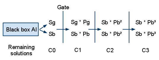
I divided the 300 tests into three gates with 100 in each. In some of my tests, no solution made it through all the gates, suggesting that I either needed more tests or more solutions, so just to test the theory I increased the number of 0.5-solutions to 100 000 and 0.6 to 50 000.

Running the solutions through the gates with a cutoff of 0.55 (meaning that we search for solutions that have a true fitness of 0.55 or better and only let those through that have a measured fitness of 0.55 on each gate) yielded the following result:

C0 = 150000

C1 = 54774 (C0 / C1 = 2.74)

C2 = 35543 (C1 / C2 = 1.54)

C2 = 27891 (C2 / C3 = 1.27)

The ratios are decreasing nicely, as expected. I solved the equations in part 1 numerically, using my genetic algorithm library, optopus, for Python, thus ending up with the following:

0.34 good solutions, with 0.82 passing through each gate

0.66 bad solutions, with 0.14 passing through each gate

This means that the predicted probability of drawing a good solution after each gate is:

0.34 (before any gate. True value is approx. 0.33)

0.75 (after one gate. True 0.75)

0.95 (0.95)

0.99 (0.99)

So in this particular special case, our method gets exactly the correct answer!

Let us make it slightly harder and choose a cutoff that is not exactly in the middle between 0.5 and 0.6.

Running the solutions as above with cutoff 0.58 (we now ask how many are equal to or better than 0.58) yielded this:

C0 = 150000

C1 = 35450 (C0 / C1 = 4.13)

C2 = 19571 (C1 / C2 = 1.81)

C2 = 11994 (C2 / C3 = 1.63)

Once again we get a nice decreasing ratio. Solving it numerically gets us these parameters

0.34 good solutions, with 0.62 passing through each gate

0.66 bad solutions with 0.04 passing through each gate

and these predicted probabilities of drawing a good solution after each gate:

0.34 (True: 0.33)

0.88 (0.88)

0.99 (0.99)

0.999 (0.999)

Ridiculously good!

Let us make it harder still and pick a cutoff above the top solutions. This violates the assumption in part 1, that we have at least one good solution.

With cutoff 0.62, I got this:

C0 = 150000

C1 = 16043 (C0 / C1 = 9.35)

C2 = 4733 (C1 / C2 = 3.39)

C3 = 1400 (C2 / C1 = 3.38)

Here something worrisome happens. The ratio stops decreasing. Since this ratio is supposed to asymptotically reach the inverse of Pg, the probability that a good solution pass the gate, this should trigger an alarm. If we say that the fitness of a good solution has to be better than or equal to 0.62 and have a cutoff of 0.62 in the gates, how can only one in 3.38 pass? We should always get at least half of the good solutions through.

Running the GA gives:

0.35 good, with a 0.3 probability to pass

0.65 bad with a 0.0004 probability to pass

Which is completely wrong, since there are only bad solutions if we try to find solutions that are 0.62 or better. Remember that all our solutions have a true fitness of 0.5 or 0.6. We again get a stern warning that something is wrong, since a 0.3 probability to pass is too low. We expect at least half of the good solutions to pass. More than half should pass if the solutions are noticeably above the cutoff value, but anything under 0.5 means we are in trouble.

Taking that warning into account, it would seem that the gate test worked here as well.

The problem

Does it always work? Sadly, no. As I hinted in my last post, there is a problem. Let us say that instead of two kinds of solutions, 0.5 and 0.6, we have 100 solutions distributed evenly between 0.3 and 0.7. Just sending this solution distribution through the 300 tests yields (15 bins):

The distribution does not look very uniform anymore, but at least it looks like we have nothing over 0.7, which is true.

With cutoff 0.65, we get:

C0 = 40000

C1 = 4656 (C0 / C1 = 8.59)

C2 = 2385 (C1 / C2 = 1.95)

C3 = 1392 (C2 / C1 = 1.71)

Everything looks all right. Running the GA gives:

0.17 good, with a 0.58 probability to pass

0.83 bad with a 0.18 probability to pass

0.17 (True: 0.13)

0.87 (0.68)

0.99 (0.85)

0.999 (0.93)

As can be seen, the algorithm overestimates how many good solutions there are. This happens because one of our initial assumptions, that there are only either good or bad solutions, is wrong. Since the C-ratios decrease, it looks like we get progressively more and more good solutions, which we are, but at a smaller rate than indicated. What happens is that the better a solution is, the more likely it is to survive, so the gates make sure that the better of the bad solutions survive, which makes a larger ratio of the entire "population" of solutions survive each time.

Note that the answer will not always be overestimated. If the even distribution is located mainly to the right of the cutoff, I think that the answer will instead be underestimated, but I have not yet tested this. It might be worth mentioning that running with cutoff 0.72 yielded very bad C-ratios, so that still works as before.

Gates as transfer functions

A series of test cases and a cutoff value can be seen as a transfer function on the distribution of solutions. When the solutions are run through a gate, the transfer function is convolved with the solution distribution to yield a new solution distribution. In the graph below, I have plotted the transfer functions for five different gates, with the same cutoff but with different number of test cases. Once again we have relatively few test cases, but just as we discussed earlier, if the test cases are not divided 50/50 between positive and negative or there are weights, we need many more to get the same gate characteristics.

The more test cases that the gate has, the steeper the transfer function. It will look more and more like a step function as the gate gets "larger". In the limit that is actually is a step function (with infinitely many test cases), our earlier assumption fully holds and the predictions would again be correct. These transfer functions will move the solution distribution to the right (better true fitness). The only thing we can measure is still C, the number of solutions left, which in the continuous case would be the integral of the solution distribution.

Possible solutions

If we knew the shape of our initial solution distribution and the shape of the transfer function, we would once again be in business and be able to predict the number of solutions above a cutoff correctly. The transfer function can be estimated, but the solution distribution can vary greatly. Maybe all solutions have the same true fitness? Maybe they are divided into two "pillars" as in the example above? Maybe they are spread in some more complex shape across the spectrum?

Instead of just finding out the value of two points of the solution distribution (good and bad), we would get better estimates if we could get the value of more points. But knowledge of more variables require more equations. Where will these equations come from? We have two sources of untapped information.

First of all, we have not used the exact result when the solutions are run against the test, only if they pass the cutoff or not. By letting the cutoff move from 0 to 1 and running the same gates over and over again, we can gain additional information on the shape of the solution distribution. If the transfer functions where linear, we would not gain additional information from this, but since they are not, the different resulting integrals can tell us something.

The results of the different cutoffs are of course not totally independent, so each new cutoff will not magically bring about a new independent equation, but it will still improve our understanding of the shape of the solution distribution.

The other source of information that we have not used is that not all solutions run against all test cases, since we filter out so many after each gate. This means that there are tests (thus information) that are not being used. The easiest way to use this information is to do as suggested in part 1 and rerun the gate experiment with the gates in different order. This will not give more equations, but will increase the accuracy of the measured Cs which in turn may allow more gates with fewer tests in each, which gives more equations.

This is my main approach and the one that I will test in practice and write my next post about.

I have, however, two other rough ideas that one could pursue.

One approach is to abandon gates and look at the measured fitness histogram for all test cases (like the two I have shown above) and try to run it in reverse, by generating hypothetical true distributions and see how likely they are to end up in the measured distribution after the blurring effect of the test process. Maybe image deblurring techniques such as Gaussian noise reduction can be used?

The other approach is to study deconvolution - the process of running a convolution in reverse. According to the Wikipedia article, deconvolution is often associated with image processing, where it is used to reverse optical distortion. Maybe this method will actually converge with the deblurring approach?

Confident optimization using gates

When dealing with any non-linear optimization or classification algorithm, like Genetic Algorithms, Artifical Neural Networks or Simulated Annealing, you need a way to compute the fitness of your candidate solutions. These algorithms all work in roughly the same way - you generate a solution, test it and generate new solutions based on feedback from the testing (the feedback will usually just consist of a fitness value).

For some problems you can get the true fitness of a solution. If you, for example, are maximizing a known mathematical function of many variables, you immediately know exactly how good your solution is. However, for most interesting problems you will never know the true fitness. If you are evolving parameters for a poker playing program, a stock predictor or a walrus image classifier, you never know quite how good your solution is in general. The best you can do is try your solution on a number of test cases and assume that your average performance on those tests are the same as your average performance when the number of test cases approach infinity.

An optimization algorithm will often become over-specialized in the test cases that it is trained on. To combat this, a method called "holdout validation" is often used. The data is divided up into several disjunct sets - a training set used for fitness calculation of the millions or billions of proposed solutions, a validation set for validating the fitness of solutions that are candidates of being the most promising so far and a test set for testing the final solution of your run. Often you will make several runs of your optimization algorithm with different types of inputs and parameters. The test set is used to decide which of the runs produced the best solution.

This standard approach will sometimes work, but there are problems. If your fitness function is very volatile and test cases are hard to come by, you can never be quite sure how consistent your solution is. What is the chance that a solution will happen to get lucky on all three sets of test cases? Low? If I am persistent and keep running the same optimization problem on my computer cluster with the inputs prepared differently and different parameters until I get something that finally pass my tests, what are the risk that after billions and billions of tries, I have just found a fluke that will not perform well on further data? Obviously one can never be completely sure, but it would be nice to at least know what the probability is that we have found a real solution.

One possibly more effective way of using your data is to employ cross validation, but if you test several solutions, the problems with "luck" will reappear.

I'd like to explore a different theory that I have been tinkering with.

Gates - an introduction

In this introduction, I will make a number of simplifications, assumptions and ungodly approximations. I hope to remedy this in the next post.

Let us take the problem of walrus image recognition from the introduction. Imagine that we have a number of subaquatic images. Half of them depict sea weed, lobsters and whatnot and half are of walruses. A good walrus classifier will identify over 70% of the images correctly.

Let us further make the assumption that a walrus classifier is either good or bad, with nothing in between. This assumption can not be entirely true, since an optimization algorithm needs a way to arrive at its solution through gradual improvement, which means that there must be somewhat good solutions. Nevertheless, it will have to do as an approximation for now.

Assume we have a black-box algorithm that spits solutions at us. We will call the number of good solutions at a certain time Sg and the number of bad solutions Sb. The total number of solutions, C0, is just C0 = Sg + Sb.

Take the images that the algorithm did not get to see and divide them randomly into three equally large sets. Each set is now a Gate, which will let through only those solutions that can correctly classify above 70% (it does not have to be the same as our target percentage) of the images in the set. We can assume that it is approximately equally hard to get through any gate. This assumption can be tested by simply sending our solutions through each gate and check that roughly the same number of solutions pass.

Unfortunately there is a chance that a bad solution could get lucky and pass the gate (a false positive) or that a good solution could get unlucky and fail (a false negative), but for a meaningful test, a good solution must always have a better chance to pass the gate than a bad solution.

Let us define the probability that a good solution passes a gate as Pg and the probability that a bad solution passes as Pb. As the number of test cases in each gate approaches infinity, Pg will approach 1 and Pb will approach 0.

If we set up an experiment where we first send our solutions through the first gate, then send the survivors through the second and finally those survivors through the third gate, we can measure the remaining population size at four points. After the black box: C0, after the first gate: C1, second gate: C2 and third gate C3.

If our gates are testing anything relevant and our population consists of both good and bad solutions (Sg != 0 and Sb != 0) we can immediately see that the ratio between successive gates should decrease C0/C1 > C1/C2 > C2/C3, because there will be a greater ratio of good solutions to bad solutions after each gate and Pg > Pb. In plain English - a smaller percentage of the solutions should disappear each time, as the population gradually contains more good solutions. If this does not hold, we must either have bad gates (too few test cases or something) or no good solutions or no bad solutions. As the ratio of bad to good solutions decrease, C(i) / C(i+1) will approach Pg as most solutions will be good.

Fortuitous results

The number of good solutions that remain after the first gate is Sg * Pg and the number of bad is Sb * Pb. Thus we get four equations:

C0 = Sg + Sb
C1 = Sg * Pg + Sb * Pb
C2 = Sg * Pg² + Sb * Pb²
C3 = Sg * Pg³ + Sb * Pb³

Since we have four equations and four unknowns, Sg, Sb, Pg and Pb, we should be able to solve what the ratio of good to bad solutions is and what the characteristics of the gates are. Subsequently we can tell what the chance is that we pick a good solution if we randomly pick one after a certain number of gates. We can also tell how many solutions we will need to generate on average until we have at least one solution that passes through a certain number of gates.

There is nothing magical about three gates. If we use more gates with fewer tests in each (thus making Pg and Pb closer) we will get different characteristics. This will result in more equations and the variables will be overdetermined, but they can still be determined using, for example, a least-squares fitting. Trying different number of gates and different gate sizes can help us find the optimal use of our test cases.

It is important that Pg and Pb are roughly the same for each gate, in other words that one gate is not significantly harder or easier to pass through than the others. If the gate sizes are large this is more likely to be true. It is straightforward to test this assumption. You can either:

• Do the simple test described earlier, making sure that C is roughly the same for each gate.
• Put the gates in different order and re-run the experiment, verifying that the results are the same.
• Run the experiment several times, dividing the test cases into three entirely new gates each time and determine the standard deviation of the calculated parameters.

If C is not roughly the same for each gate, you need larger gates. Go find more data or use fewer gates, but no fewer than three. That simple. (Almost.. we have not defined exactly how rough "roughly" is)

Caveat
So.. Is everything solved that easily? Can we now go out and confidently optimize the world as the title suggests? No, but I believe this approximation can be of great use as it stands. Earlier we made the assumption that solutions are either good or bad, instead of somewhere in a continuous fitness spectrum. In my next post, I will explain why this makes things a bit more complicated.